Market Basket Analysis on Chronic Systolic
Heart Failure Prescribing
A Penn State DAAN 888 capstone applying association rule mining, dimensionality reduction, and time series forecasting to a real IQVIA longitudinal prescription dataset for Chronic Systolic Heart Failure (HFrEF, ICD-10 I50.22, ejection fraction ≤ 40%). Roughly 6.7 million Americans are diagnosed with heart failure annually, about half with reduced ejection fraction. The project started from a simple question, prompted by how many heart-drug TV ads exist: which drugs actually get prescribed together, and what does that pattern reveal about clinical practice, drug clusters, and future prescribing volume?
The IQVIA Prescribing Dataset
The source is IQVIA's longitudinal U.S. prescriber-level dispensing data for Chronic Systolic Heart Failure. Each row in the raw wide-format table is an aggregated count of prescriptions for a unique combination of drug, manufacturer, specialty, age band, gender, and month/year, with a total_count column holding the number of prescriptions. To make the data compatible with market basket analysis, rows are exploded into one transaction per visit — duplicating each row total_count times — which expands the table to 7,685,672 rows × 9 columns.
| Column | Type | Scale | Example |
|---|---|---|---|
| Month, Year | DateTime | Interval | August 2019 |
| Manufacturing Company | String | Categorical | Accord Healthcare |
| Drug Name | String | Categorical | Eplerenone |
| Type of Drug | String | Categorical | Addiction Medicine |
| Age Range | String | Ordinal | 65 to 74 |
| Gender | String | Categorical | Male |
| ICD-10 Code | String | Constant, dropped | I50.22 |
| Description of Disease | String | Categorical | Chronic Systolic Heart Failure |
| Number of Visits | Integer | Ratio | 150 |
Storage & Traversal Architecture
The pipeline is designed to handle over ten million records: raw JSON lands in MongoDB as a schema-less staging area, Hadoop/HDFS and Spark run distributed ETL, curated time-series records move into Cassandra for high-availability writes, a summarized analytical subset is loaded into PostgreSQL for BI querying, and Redis caches frequently-requested aggregates ahead of Power BI dashboards.
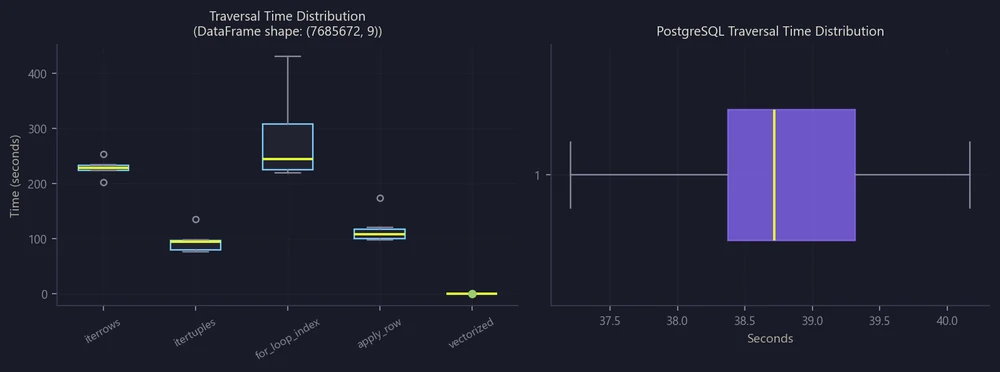
itertuples is fastest (~88s median), followed by apply (~115s), iterrows (~228s), and plain index-based for-loops, the worst at ~262s. Querying the same scale through a PostgreSQL cursor lands at a consistent ~37–40s, useful when server-side filtering can reduce what's transferred client-side.Market Basket Analysis of Co-Prescribed Drugs
Market basket analysis uncovers purchase patterns — here, prescribing patterns — using association rule mining to find drugs that frequently co-occur within the same patient visit. The project set out to answer four questions: which drugs are commonly prescribed together for a given age range and gender; when a specific drug class is prescribed, what other classes accompany it; which competitor products land in the same "basket" for the same underlying condition; and whether similar drugs are prescribed across ostensibly unrelated specialties, such as addiction medicine and cardiology.
total_count) is expanded into one row per individual visit, duplicated total_count times per combination — converting the wide-format table into the 4.5M-row transactional format used for FP-Growth-style association mining.Top Co-Prescribed Pairs by Year
| Year | Top Pair | Co-occurrences | Support | Confidence |
|---|---|---|---|---|
| 2019 | Carvedilol ↔ Metoprolol Succinate | 213 | 11.59% | 44.84% |
| 2020 | Carvedilol ↔ Metoprolol Succinate | 568 | 12.82% | 49.48% |
| 2021 | Carvedilol ↔ Metoprolol Succinate | 584 | 13.50% | 50.87% |
| 2022 | Carvedilol ↔ Metoprolol Succinate | 585 | 13.46% | 46.54% |
| 2023 | Metoprolol Succinate ↔ Spironolactone | 549 | 12.53% | 31.23% |
| 2024 | Carvedilol ↔ Metoprolol Succinate | 630 | 14.96% | 55.17% |
| All years | Carvedilol ↔ Metoprolol Succinate | 1,034 | 18.14% | 63.79% |
From PCA to t-SNE to TruncatedSVD
Before clustering, categorical fields (drug, manufacturer, specialty, age range, gender) are numerically encoded, and three dimensionality reduction techniques are compared year-over-year to find the one that best preserves structure in this high-dimensional, largely categorical pharmaceutical data.
| Year | PCA Variance Explained | t-SNE Variance Explained |
|---|---|---|
| 2019 | 0.301 | 0.58 |
| 2020 | 0.292 | 0.62 |
| 2021 | 0.356 | 0.47 |
| 2022 | 0.399 | 0.59 |
| 2023 | 0.401 | 0.54 |
| 2024 | 0.391 | 0.55 |
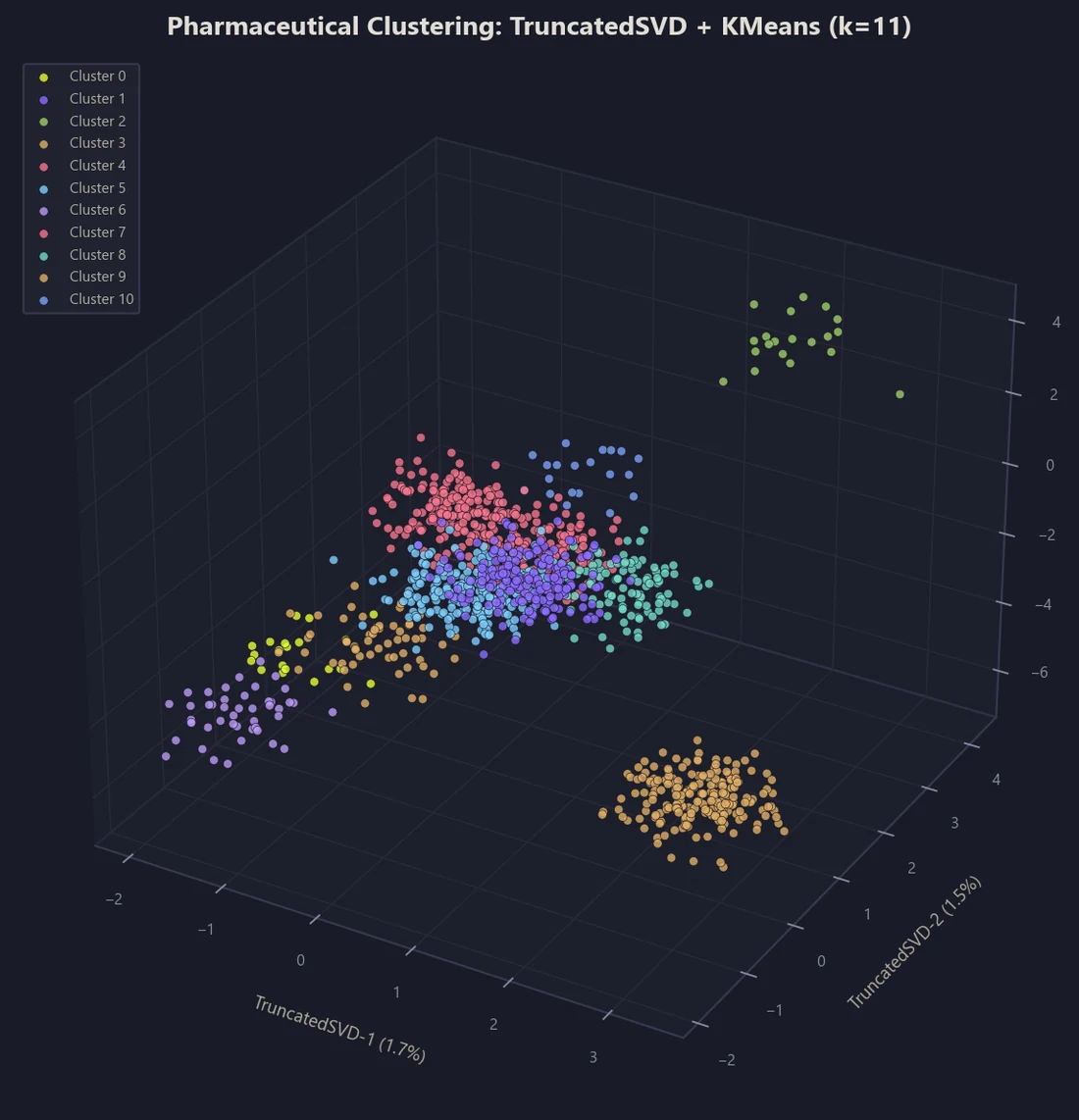
PCA averages only ~37% variance explained — it captures linear relationships well but misses the fine-grained local structure this categorical data needs. Moving to t-SNE lifts average variance to ~58%, but it fluctuates between 0.47 and 0.62 across years with no stable global representation, making clusters hard to interpret quantitatively. TruncatedSVD resolves both problems: three components capture 80% of total variance, and the resulting space is stable enough to cluster reliably.
Predicting Clusters, Drugs, and Gender
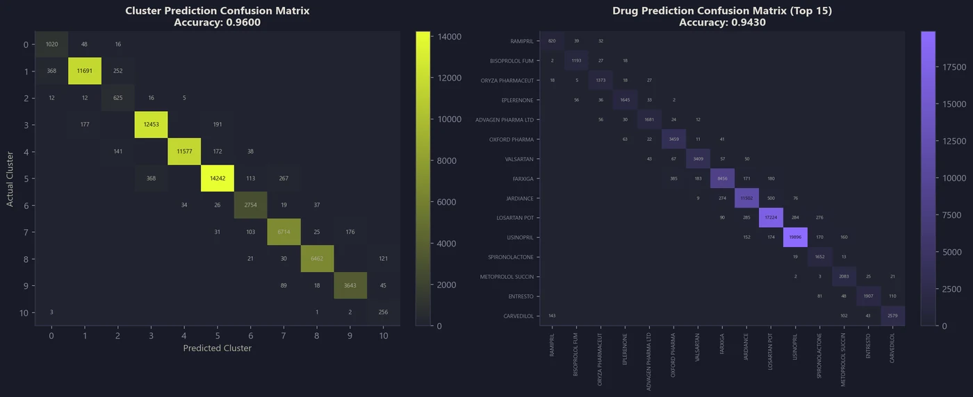
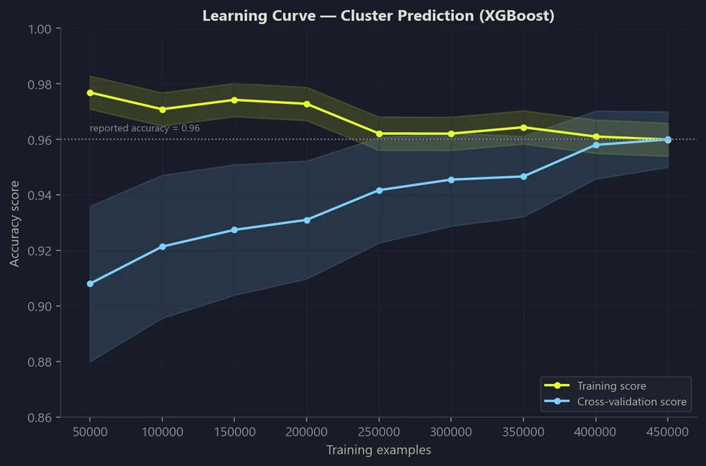
To validate that the unsupervised clusters were meaningful (not artifacts), an XGBoost classifier was trained to predict cluster membership and drug identity directly from the SVD components. A separate pipeline — Random Forest, SVM, and Gradient Boosting — tests whether prescribing patterns alone (no demographic fields) can predict patient gender.
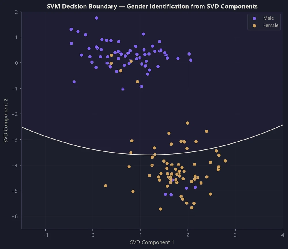
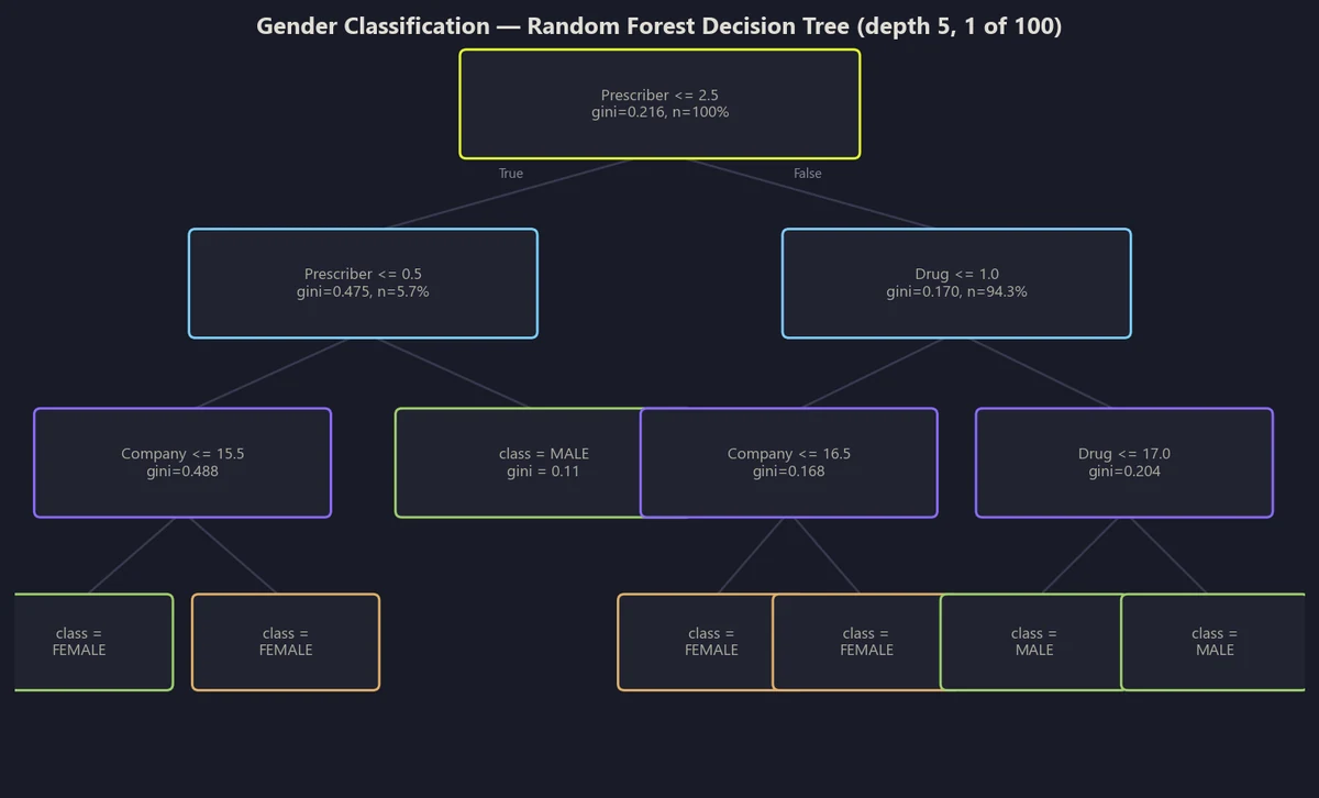
Prescriber is the strongest gender differentiator in both trees — the very first split — with terminal-node gini values near zero, meaning gender is discoverable through fairly simple decision rules from prescribing behavior alone.Seven-Stage Forecasting Pipeline with Synthetic Augmentation
Forecasting monthly prescription volume runs into a hard constraint: only a handful of complete annual cycles exist, which starves data-hungry models. Rather than accept that ceiling, the pipeline generates synthetic training data through three different techniques before feature engineering and modeling.
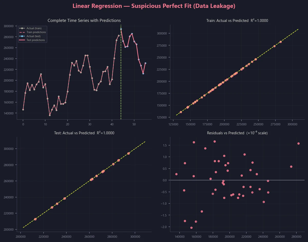
Synthetic data is generated independently per train/validation/test split to avoid leakage — the same principle that caught the linear regression bug in the Results section.
GAN — "Mimic"
A Generator and Discriminator train adversarially until the Generator produces sequences the Discriminator can't distinguish from real data. Flexible and expressive, but training can be unstable (mode collapse, vanishing gradients) and computationally heavy.
DTW — "Time Warping"
Dynamic Time Warping finds the optimal temporal alignment between similar sequences and synthesizes new data by morphing between them. Preserves temporal coherence well, but can only interpolate within the convex hull of existing patterns — limited novelty.
TSGM — "GAN + Encoders"
An Encoder-Decoder-Discriminator architecture with recurrent/attention layers, purpose-built to preserve autocorrelation and seasonality. Generally more stable than a plain GAN, at the cost of added architectural complexity.
Feature engineering converts the cleaned time index into month_sin/month_cos cyclical encodings, lag_1/2/3 autoregressive terms, 3-month rolling mean/std/max, yearly growth, and 1- and 3-month momentum — giving every model family the same seasonal and trend signal to work with.
Forecasting Results — and an Honest Data Leakage Catch
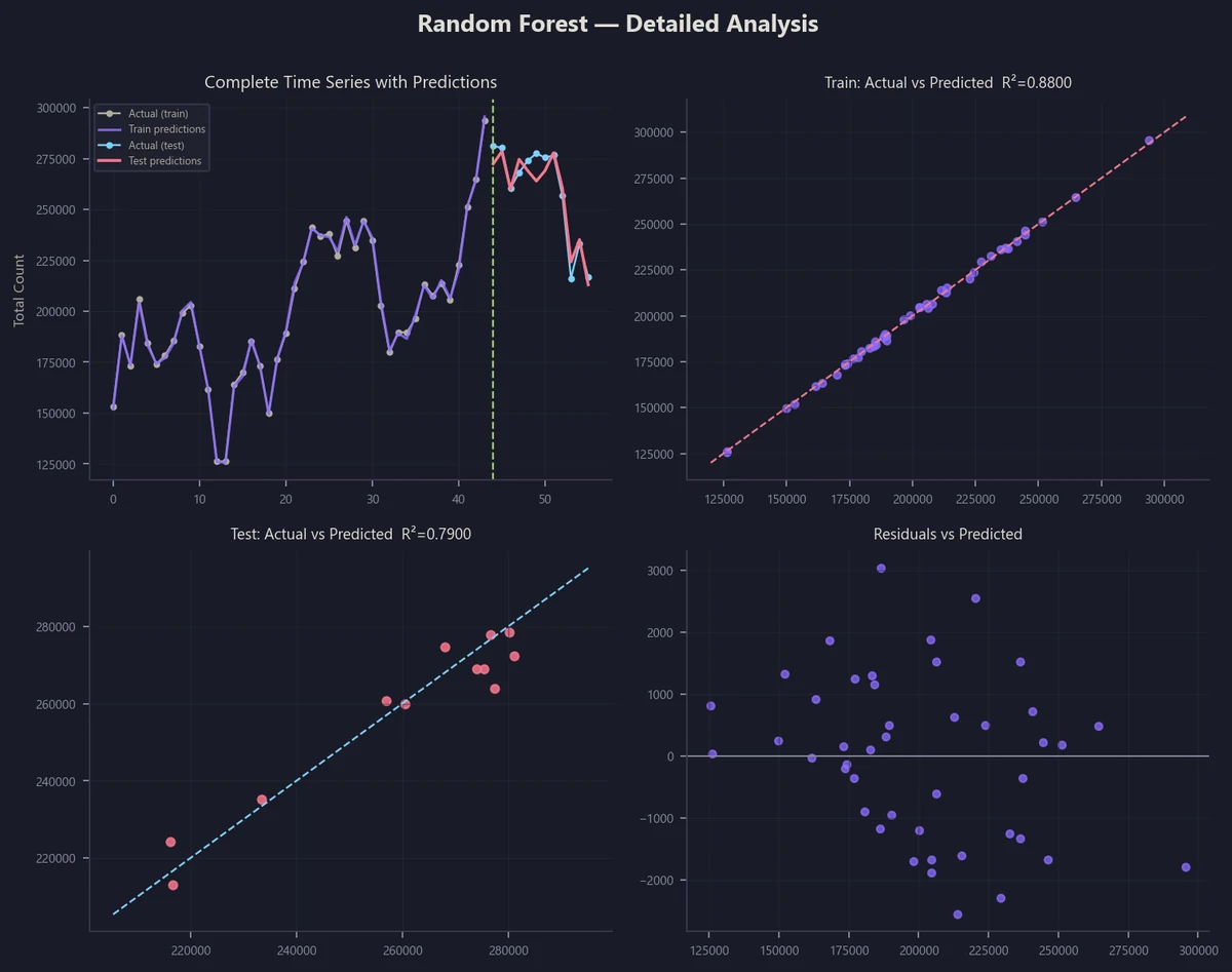
Four model families were evaluated on both the original and GAN/DTW/TSGM-augmented training data. The most useful result of this section wasn't the best score — it was catching a bad one.
Linear Regression: R² = 1.0000 is a red flag, not a win
The baseline linear/ridge regression achieved a perfect R² of 1.0000 on both training and test sets, with residuals at the 10-10 scale — floating-point noise, not real error. No legitimate model achieves perfect prediction on real-world time series. This is a textbook sign of data leakage: either the target leaked into the features, or the train/test split preserved temporal information it shouldn't have. Rather than reporting this as a strength, the report flags it explicitly as a methodology bug requiring investigation — and excludes it from the model comparison that matters.
| Model | Train R² (original) | Test R² (original) | Train R² (augmented) | Test R² (augmented) |
|---|---|---|---|---|
| KNN | 1.00* | ~0.14 | 1.00* | ~0.91 |
| Random Forest | 0.88 | 0.79 | 0.97 | 0.88 |
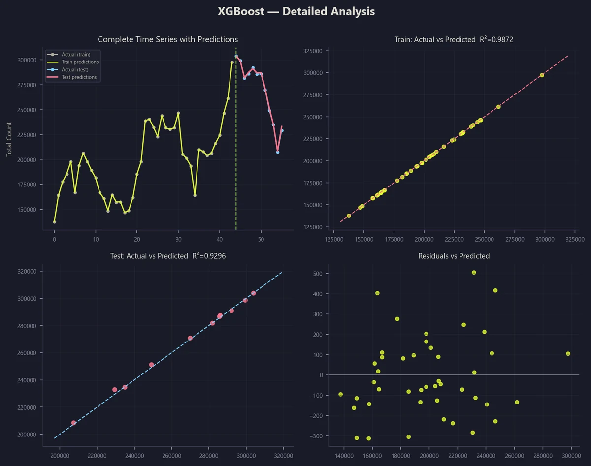
| XGBoost | 0.9872 | 0.9296 | 0.99 | 0.97 |
*KNN's train R² of ~1.0 reflects memorization of training points, not genuine fit — its collapse to ~0.14 test R² on original data confirms it. Augmentation lifts KNN's test score but the residuals stay large and noisy, suggesting it's fitting injected synthetic patterns more than real structure.
Key Findings
Carvedilol + Metoprolol Succinate is the top co-prescribed pair in five of six years (confidence 45–55%, reaching 63.79% across all years combined) — consistent with guideline-directed dual beta-blockade for HFrEF.
Dapagliflozin and Jardiance appear as high-support MBA pairs (28–29%) starting in 2024, tracking the ~2-year lag between SGLT2 inhibitors' expanded FDA heart-failure indication and adoption in prescribing practice.
TruncatedSVD captures 80% of variance in 3 components versus PCA's ~37% average and t-SNE's inconsistent 47–62% swing — the deciding factor in choosing it for the k=11 KMeans clustering.
Random Forest and SVM classify patient gender from prescribing patterns alone — no demographic fields — with Prescriber as the single strongest differentiator, the root split in every decision tree.
96% cluster accuracy, 94.3% drug accuracy, and the best forecasting test R² (0.93 original data, 0.97 augmented) — XGBoost was the strongest model across all three problem types in this project.
A baseline linear model returning a perfect R² = 1.0000 was flagged as a methodology bug, not a result — a deliberate reminder that a suspiciously perfect score is a signal to investigate, not celebrate.